Monte Carlo vs Discrete Rate Simulation
When Is a Spreadsheet Enough?
Monte Carlo simulation is often the first tool an engineer reaches for. It fits in a spreadsheet and handles uncertainty well, but it has no clock. Here’s when that matters for manufacturing questions, and when it doesn’t.
What Monte Carlo simulation is
The Monte Carlo method was developed in the 1940s at Los Alamos, associated with Stanislaw Ulam, John von Neumann and Nicholas Metropolis. You describe each uncertain input with a probability distribution, draw one value from each, compute the result and repeat thousands of times. The results approximate the distribution of the output.
In most manufacturing and business use, Monte Carlo is static. Each trial is a separate calculation with no simulated time inside it, only a formula.
What a dynamic simulation adds
A dynamic simulation has a clock and a state that evolves. The level in a buffer at 10:05 depends on its level at 10:04, on whether the upstream machine was running and on whether the downstream machine was taking material. Discrete event, discrete rate and continuous simulation are all dynamic. They differ in how they move the clock, as covered in simulation methodologies.
Dynamic stochastic models also use random sampling. Failure and repair times are drawn from distributions as the model runs, and the model is replicated to get a range of results. So the real difference between Monte Carlo and a discrete event model isn’t randomness. It’s whether time and state are part of the model.
| Aspect | Static Monte Carlo | Dynamic simulation |
|---|---|---|
| Simulated clock | None | Yes, event to event |
| State carried forward | No, each trial is independent | Yes: buffer levels, machine states, queues |
| Randomness | Sampled inputs per trial | Failures, repairs and arrivals sampled during the run, plus replications |
| Buffers, blocking, starving | Can’t be represented | Represented directly |
| Build effort | Hours, in a spreadsheet | More, since it needs structure, logic and data |
| Typical output | Distribution of a total | Distributions over time: throughput, downtime, buffer behavior and where losses occur |
Where the static view breaks: two machines
Take two machines in series, each available 90% of the time. A Monte Carlo spreadsheet samples each machine’s availability and multiplies them, so on average the line is available about 0.9 × 0.9 = 81% of the time. That arithmetic holds only if every stop on either machine stops the whole line at once, and the two machines fail independently.
Now put a buffer between them. When the upstream machine stops, the downstream machine keeps running from the buffer until it empties. When the downstream machine stops, the upstream machine keeps filling the buffer until it’s full. Whether the buffer rescues a little output or a lot depends on how long the stops last compared with how many minutes of material the buffer holds. That’s a question about timing, and the formula has nowhere to put it.
The independence assumption is weaker than it looks, too. A machine that’s blocked or starved isn’t running, and many failure modes only occur while a machine runs. Stops on one machine change how often its neighbors fail. A dynamic model represents that interaction, and a multiplication doesn’t. Spreadsheet, dashboard, AI or simulation? covers the same bias in a loss tree.
When Monte Carlo is enough
- Independent risks. Project cost and schedule risk, supplier delays that add up, or several risks that don’t interact.
- One-period totals. Annual demand against nominal annual capacity, where the question is whether the volume fits at all rather than how the line behaves hour to hour.
- Separate assets. Several independent lines where a stop on one doesn’t affect another.
- Screening. A quick sensitivity check to find which uncertain inputs matter before investing in a detailed model.
When you need a dynamic model
- Buffers and accumulation between machines, and questions about how big they should be.
- Blocking and starving, where a stop on one machine spreads up and down the line.
- Short, frequent stops, where the length of each stop decides what’s lost, not just the total downtime.
- Changeovers, schedules and sequences, where the order of events matters.
- Moving bottlenecks, where the constraint shifts as machines fail and recover.
- Any “what if we change X” question where X interacts with timing, such as a faster filler, a larger accumulation table or a new maintenance plan.
Discrete rate or discrete event for the dynamic model?
Both are dynamic, and both handle the interactions above. The difference is what they count as an event. Discrete event simulation typically treats each unit as an entity, so the work grows with the number of units. Discrete rate simulation treats flow as a rate that stays constant between events, so the work grows with the number of rate changes (failures, repairs, changeovers, buffers filling or emptying). On high-speed lines that makes discrete rate a natural fit. For discrete parts with routings and attributes, discrete event is the better tool. The full comparison is in discrete rate vs discrete event simulation.
Speed matters, because every design alternative needs its own set of replications. The published example is the ExtendSim® model from Fischel and Lange’s WSC 2020 study of a food plant, which was rebuilt in ReliaSim® and independently validated by Tom Lange. The ReliaSim model came within 1% of both the plant’s measured OEE and the original model (case study).
A practical sequence. Use Monte Carlo to scope the uncertainty and find the inputs that matter. If the answer depends on timing, build the dynamic model, fit its failure and repair distributions from your own event data, validate it against history, and then run the experiments.
ExtendSim® is a registered trademark of Andritz Inc., referenced for identification only.
Frequently asked questions
Is Monte Carlo simulation the same as discrete event simulation?
No. Monte Carlo simulation is static. It samples uncertain inputs and computes a result, with no simulated clock and no state carried forward. Discrete event simulation is dynamic. It moves a clock from event to event and tracks how the state of the system changes over time. The two are often combined, because a stochastic discrete event model is run for many replications and the spread of those results is summarized in a Monte Carlo fashion.
Can Monte Carlo simulation predict manufacturing throughput?
It can give a useful first estimate when machines are effectively independent, for example separate lines, or a line with no meaningful buffers where every stop halts the whole line. Once buffers, blocking and starving, changeovers or the length of stops matter, throughput depends on timing, and a static calculation can’t represent timing. That’s when a dynamic model such as discrete rate or discrete event simulation is needed.
What is the difference between static and dynamic simulation?
A static simulation represents a system at a single point, or over a period treated as one lump, so time plays no role. A dynamic simulation represents how the system evolves over time, so the state at one moment depends on the state a moment earlier. Monte Carlo spreadsheet models are static, and discrete event, discrete rate and continuous models are dynamic.
Do dynamic simulations use Monte Carlo methods?
Usually, yes. A stochastic dynamic model samples failure times, repair times and other random inputs as it runs, and it’s replicated with different random numbers so results can be reported as a range rather than a single figure. The difference is that each replication carries state through simulated time, which a static Monte Carlo model doesn’t.
When is a spreadsheet model good enough?
When the result is a sum or product of uncertain quantities that don’t interact through time, such as budget and schedule risk, annual demand against nominal capacity, or independent failure risks. If the answer depends on what happens while a buffer drains, how long a stop lasts or the order in which things occur, a spreadsheet will give a confident answer to the wrong question.
Try a line with real downtime
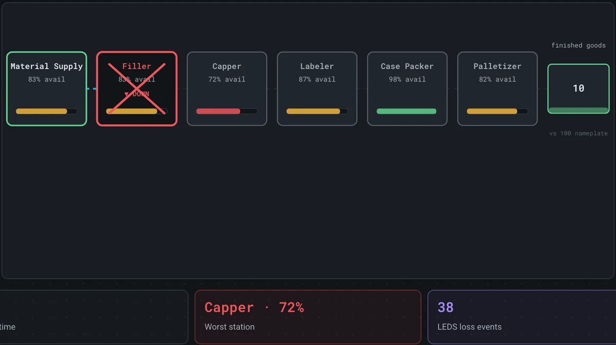
The Bottling Line demo shows why one availability number hides where the losses are.
Open the Bottling Line →Or read digital twin vs simulation.