OEE Simulation: See What a Change Does to OEE Before You Make It
From per-machine interrupt data, validated before you rely on it

Why measured OEE can't predict a change

OEE multiplies three factors (Availability × Performance × Quality) and grades execution against planned production time. It's a good scorecard. As a forecasting tool it has three structural problems, and more care with the data won't fix any of them.

• It has no history for the change. The questions worth spending money on are about things you haven't done yet, like a buffer you haven't installed or a speed you haven't run. No trend line on last year’s OEE contains them.
• Losses interact. Ten minutes down on a machine feeding a full buffer costs nothing. The same ten minutes on a starved constraint costs ten minutes of finished product, yet the OEE report records both the same way.
• Averages run optimistic. Multiplying average rates and availabilities overstates throughput, so spreadsheet forecasts of OEE come out predictably too high.

So when an improvement project promises a number of OEE points, the number usually came from subtracting a loss from a loss report. What actually comes back is often different, in both directions, as which loss to fix first explains.

Machine OEE isn't line OEE

The world-class benchmark of 85% is a single-machine figure. Carry it to a line and the topology decides what it's worth.

The real row is the one that matters, and no formula reaches it. Multiplying machine availabilities assumes the machines fail independently, and buffers break exactly that assumption. So a plant that multiplies out to 46.7% can measure 54.3%, because the arithmetic can't see the decoupling the physical line has. Is 85% OEE achievable on your line? works through the consequences.

How OEE simulation works

In ReliaSim, each factor of OEE lands somewhere concrete in the model.

The interrupt data decides accuracy. With a Line Event Data system or a historian, ReliaStats fits each failure mode’s distributions from the raw events and hands ReliaSim parameters it reads directly (downtime data analysis is its job). For a line that doesn't exist yet, the Interrupt Designer lets you enter the shapes by hand.

Named failure modes matter more than they look. One lumped downtime figure per machine still gives a working model, but the answer comes out flat, with nearly identical gains and losses, as the WSC 2020 study found. Per-mode detail lets the model tell one improvement from another.

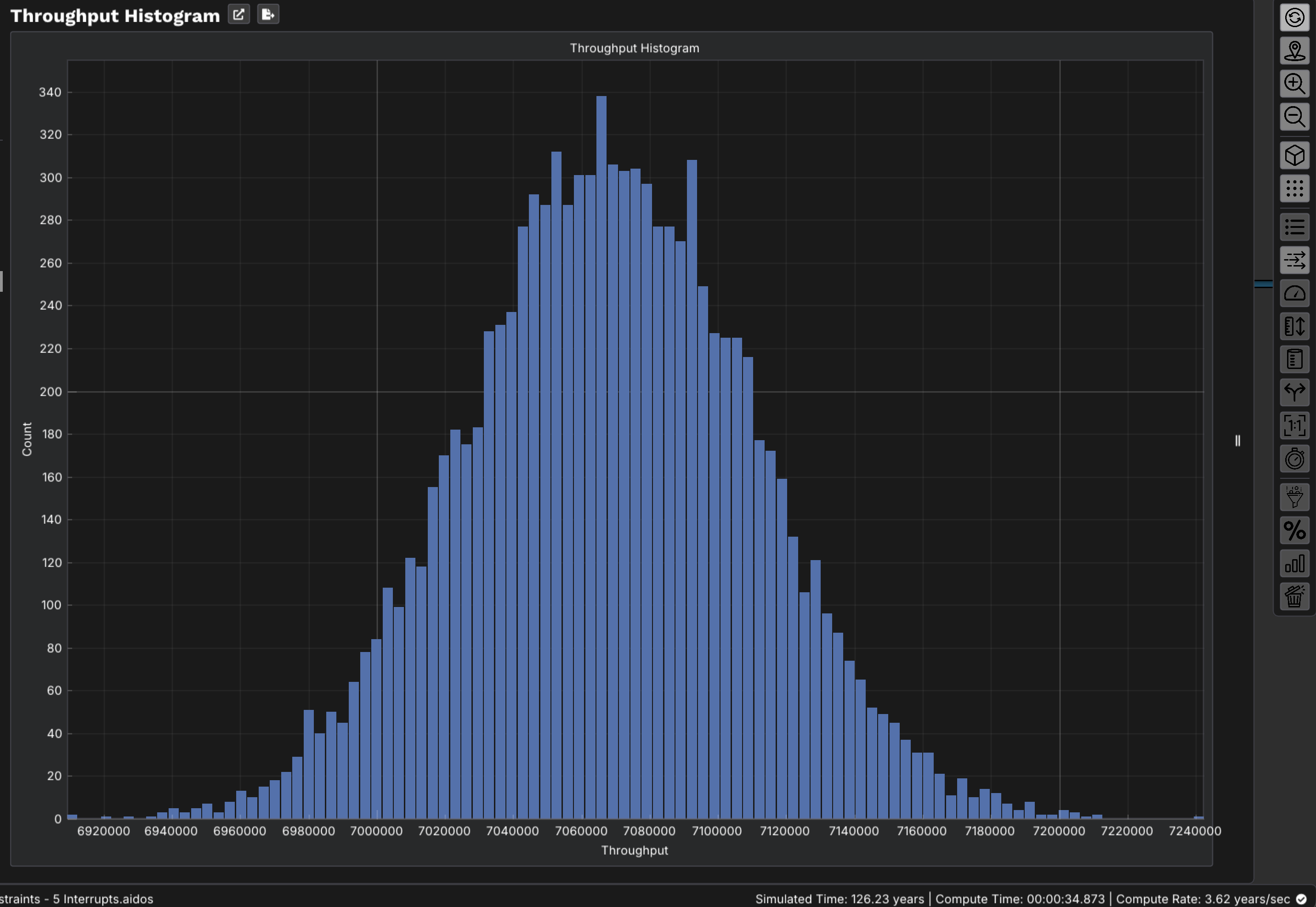
Then the engine runs the line forward through time, for a year or for many years across replications, and reports the efficiency it produced for each machine and for the line. The result is a distribution instead of a single figure, so you see the spread a single year of history can hide.

Validate against measured OEE first

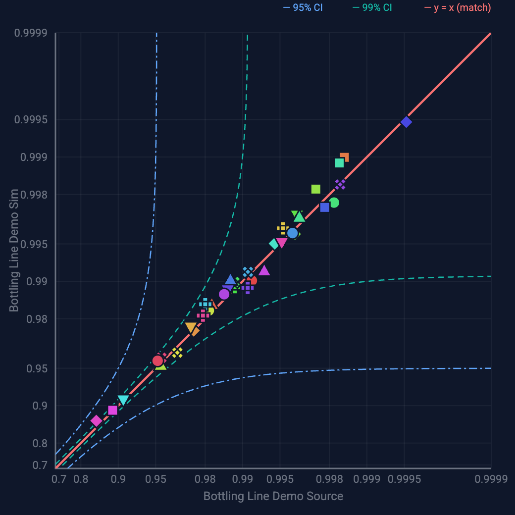
A simulated OEE is worth nothing until the model has reproduced the OEE the line actually delivered. ReliaSim holds that standard for each failure mode, not just in aggregate. Every interrupt’s simulated availability is compared with its observed availability, and each should land on the match line inside its confidence band. A single overall number can be right for the wrong reasons, with one mode overstated, another understated, and the errors canceling. A per-mode comparison can’t hide that.

At plant scale the evidence is published. A peer-reviewed multi-line food plant model came within 1% of measured OEE, and so did its ReliaSim rebuild. See the published OEE validation case study.

Simulated efficiency and your reported OEE

Put a simulated figure next to a plant dashboard and they may differ by twenty or thirty points. Usually neither is wrong. OEE divides by planned production time. ReliaSim’s efficiency uses the stricter convention and divides by every minute of the modeled period, staffed or not. On a plant that runs 24/7 the two denominators are the same and the numbers should agree. On a one-shift plant they differ by exactly the time left unscheduled.

Reconciling them is simple. Multiply the scheduled-time figure by the share of calendar time you actually scheduled, and any difference left over is about the model. Asset efficiency vs OEE covers the arithmetic, and how big is your hidden factory? covers what the gap is worth.

What you can predict

Once the model reproduces the line, every question becomes the same experiment. You change one thing, re-run, and compare.

• Remove a failure mode. The OEE that comes back isn't the loss the report recorded. Some modes return less because a buffer was already absorbing them, and others return more because they were cascading downstream (micro-stops vs breakdowns).
• Resize a buffer. Sweep capacity and see where the OEE curve flattens (how big should a buffer be?).
• Change line speed. Running faster raises the failure rate too, so OEE and output peak at some speed instead of rising with it.
• Find the ceiling. Turn every interrupt off and the model reports the most this topology can produce, so you know how much OEE is actually available to recover.

Deciding which of those improvements to fund, and what each trades away, is its own question, covered in OEE improvement tradeoffs. This page covers the tool that prices them.

Runs are cheap enough to compare every candidate instead of the three someone nominated. It all runs in ReliaSim’s manufacturing simulation software on your own desktop, and the discrete rate simulation engine makes that speed possible.

Frequently asked questions