OEE Improvement
Every Fix Is a Tradeoff
Most advice on how to improve OEE is a list: cut changeovers, fix breakdowns, eliminate minor stops, run at rated speed. Every item on it is sensible, and every item trades against something else on the line. The plants that raise output, rather than just the metric, are the ones that price the tradeoff before they spend.
Why a list of fixes is not a plan
OEE is Availability × Performance × Quality, and the Six Big Losses map onto those factors: equipment failure and setup onto Availability, minor stops and reduced speed onto Performance, process defects and startup yield onto Quality. That structure invites treating each loss as an independent lever — pull it, and OEE rises by its share.
The levers are connected. Speed changes failure rates. Buffers change what a stoppage costs. A machine’s OEE and the line’s output are different quantities. And the metric itself can move because the schedule changed rather than the equipment. Five tradeoffs come up on nearly every line, and two experiments price most of them.
Tradeoff 1: speed vs stops
Performance loss is the gap between actual and rated speed, so the obvious fix is to run faster. On many machines, running faster also means more jams, misfeeds and minor stops — failure rate rises with rate. Performance goes up, Availability comes down, and output follows whichever moved more.
This is not hypothetical. Fischel and Lange’s published model of a food plant, in which each unit operation’s failure rate scaled with its production rate, found that throughput has an optimum rather than rising steadily with speed. Any analysis that treats rate and reliability as separate numbers cannot see that optimum, let alone locate it.
Tradeoff 2: downtime vs buffer capacity
On a loss report, downtime is downtime. On the line, what it costs depends on where it happens. Ten minutes down on a machine feeding a well-stocked buffer can cost almost nothing, because the machine downstream keeps drawing on stock. The same ten minutes on a starved constraint costs ten minutes of finished product.
So two levers compete: add storage so stoppages stay local, or make the machine stop less. Both raise output, and they cost very different things. Storage costs capital, floor space and work-in-process — and in food and beverage, shelf life, sanitation time and recall exposure as well. Reliability work is often harder, but it compounds: fixing a failure helps every machine downstream at once. The published literature notes that where space is available, buffer capacity can be the cheaper lever; in many plants that qualifier carries most of the sentence. The full argument is in How big should a buffer be?
Tradeoff 3: machine OEE vs line OEE
The 85% world-class figure is a single-machine benchmark. Five machines at 85% in series with no buffering give a line near 44% (0.855); with unlimited buffering, 85%. Real lines land between, and where depends on topology and buffering, not on any one machine. See Is 85% OEE achievable on your line?
The corollary for improvement work: raising a machine’s OEE raises line output only to the extent that machine’s losses were reaching the end of the line. A machine whose stops a buffer already absorbed, or which spent its time starved or blocked by something else, can post a better number while the line makes exactly the same product. And the machine that limits the line is not fixed — it moves with downtime, product mix and schedule, which is the subject of theory of constraints simulation.
Tradeoff 4: changeovers vs responsiveness
Setup and adjustment is an Availability loss, and the direct way to cut it is to change over less often: longer runs, fewer format changes. That trades changeover time for inventory and for responsiveness to the order book. Faster changeovers trade engineering effort instead, and what they return depends on where the changeover sits relative to the constraint. At Bell-Carter Foods, two-hour changeovers on the pitting machines made them look decisive; the binding constraints turned out to be downstream in packaging (case study).
Product mix has a second-order effect a loss report cannot show: it can move the bottleneck. On a Make-Store-Pack coffee operation, changing the packaging size relocated the constraint, and a planning system that assumed a fixed constraint could not schedule it until a rate-based model reproduced the behaviour (The Shifty Bottleneck).
There is a tradeoff inside the metric, too. OEE is measured against planned production time, so it can be improved by scheduling less: cut a shift and availability against plan goes up while the asset produces no more. Nobody has to be gaming anything for that to happen. Measure against the full calendar as well — see Asset Efficiency vs OEE — and the capacity you chose not to schedule, the hidden factory, becomes visible.
Tradeoff 5: maintenance spend vs recovered throughput
Maintenance and reliability budgets are usually allocated from a downtime Pareto, largest bar first. That ranks losses by minutes, which measures how often and how long something stopped — not whether the line noticed.
Two patterns keep reversing that ranking. Frequent short stops tend to cost more than their minutes suggest, because on a tightly coupled line they never let buffers refill and they cascade into neighbouring machines. Long stops on a buffered machine often cost less, because storage absorbed part of them. The spend question is therefore not “what lost the most?” but “what comes back if we fix it, and what does the fix cost?” Only the second question produces a number you can set beside a budget line.
Loss/gain analysis: ranking losses by what comes back
Loss/gain analysis answers that question directly. In a validated model of the line, disable one interrupt — one failure mode — re-run the whole line, and measure the production recovered. Repeat for every interrupt. Each failure mode then carries two numbers: its loss, the share of time it was down, and its gain, the output that returns when it is removed.
The two disagree, and the disagreement is the finding. A gain larger than the loss means the failure mode was cascading into other machines. A gain smaller than the loss means a buffer, or another interrupt, was already absorbing part of it. On the Buffer-Options bottling-line demo over a 90-day, ten-replication run, the Labeler misalignment reads a loss of 6.67% and a gain of 4.85%. In our bottling line case study, two failure modes with near-identical losses recovered 1.21× and 0.73× their loss.
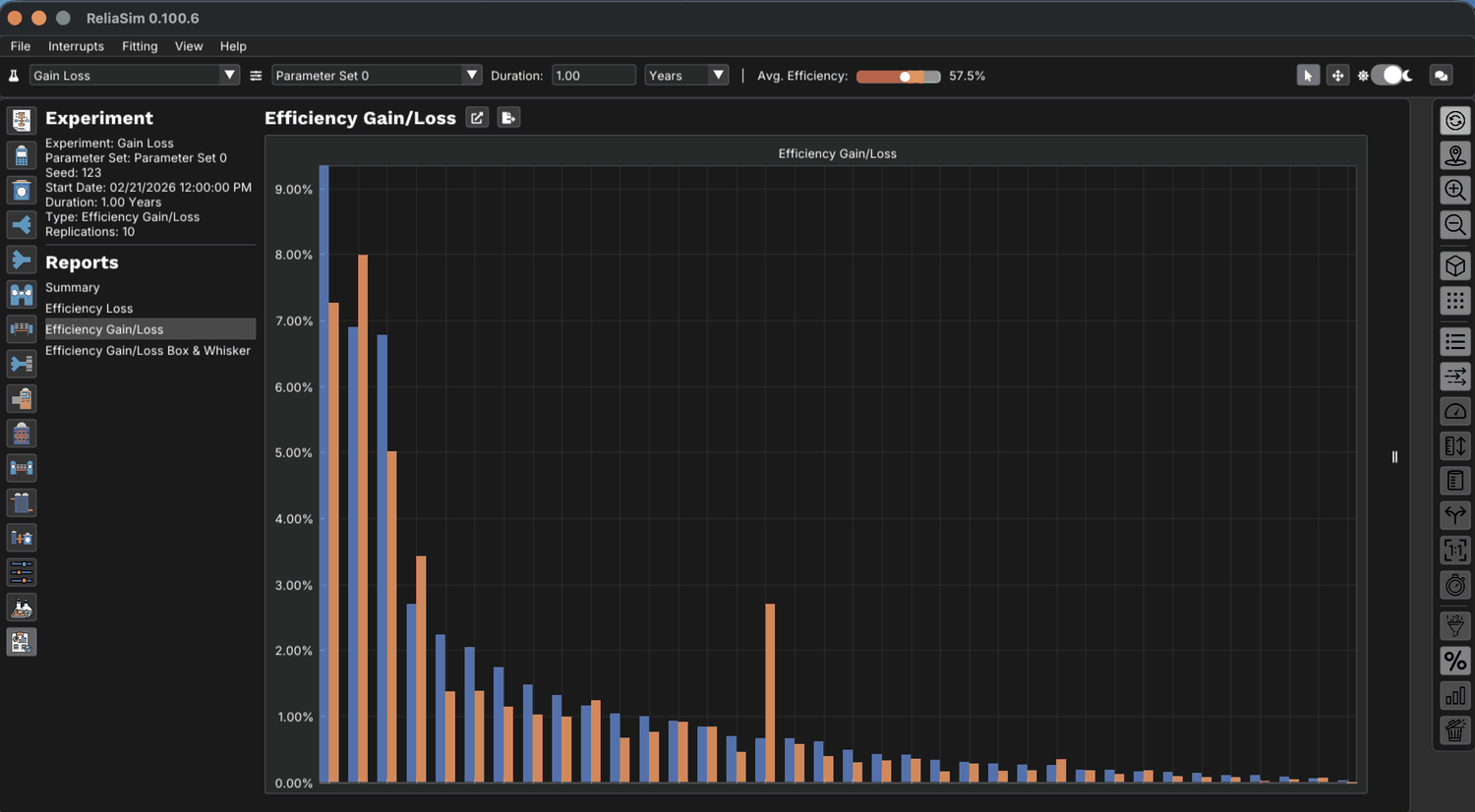
In ReliaSim this is the Efficiency Gain/Loss experiment, and a reference version for the bottling-line demo models is available on ReliaSim’s public MCP server. Its value depends on failure-mode detail: Fischel and Lange note that an averaged, single-failure-mode-per-operation model would have made the gains and losses “essentially identical to each other” — which erases the ranking entirely. The method in full is in Which loss to fix first.
Buffer tradeoff: where more storage stops paying
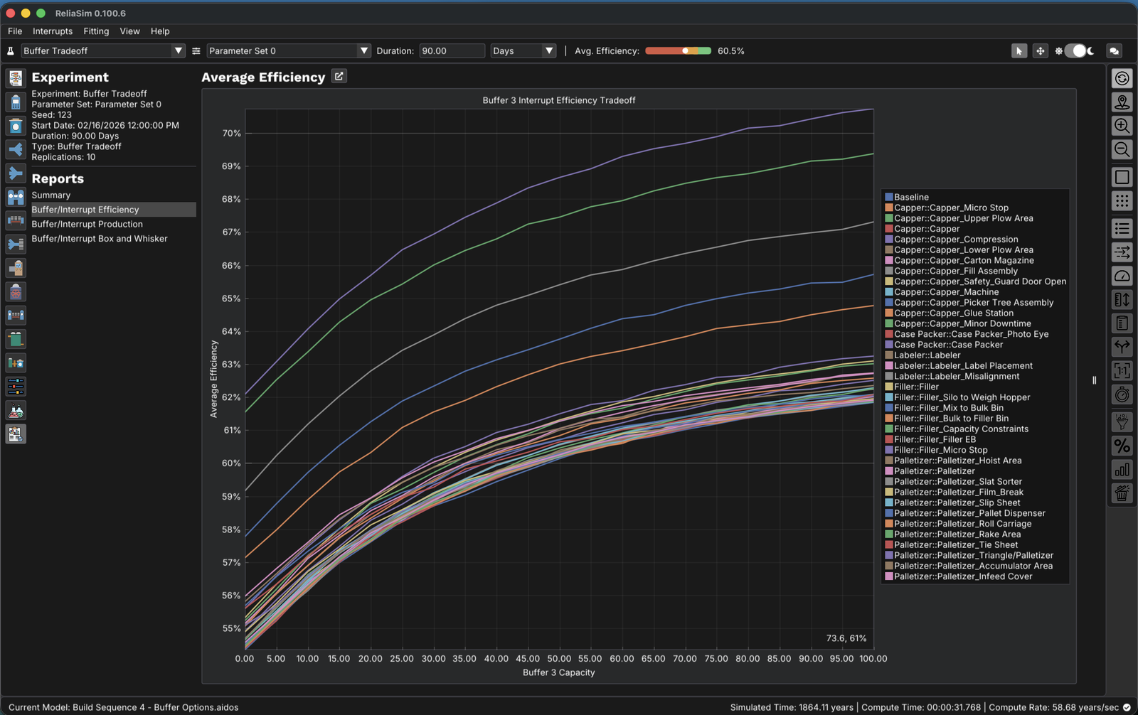
The buffer tradeoff experiment prices tradeoff 2. It sweeps a buffer’s capacity across a range while selectively dropping interrupts, so added storage and removed downtime can be read on the same axis (Buffer Tradeoff results in the docs).
The curve has the same shape on every line: efficiency rises steeply while the buffer is covering common, short stoppages, then flattens as it reaches for rare, long ones. The knee is where extra capacity stops buying throughput; past it you are buying work-in-process. Where the knee falls — and whether removing an interrupt beats any amount of storage — is specific to the line.
Pricing the tradeoffs before you spend
Every tradeoff above has the same structure: two levers that both raise some number, costs you already know, and a throughput effect you do not. The throughput side is what OEE simulation supplies — provided the model deserves trust.
The five tradeoffs, and how to price each
| Lever | What it improves | What it can cost | How to price it |
|---|---|---|---|
| Run faster | Performance | Availability, if failure rate rises with speed | Model failure rate tied to rate; compare speeds |
| Add buffer capacity | Output through short stops | Capital, space, WIP, shelf life | Buffer tradeoff |
| Raise one machine’s OEE | That machine’s number | No line gain if its losses were absorbed | Starved/blocked time; constraint timeline |
| Fewer changeovers | Availability | Inventory, responsiveness | Model the schedule and the mix |
| Fix the biggest downtime bar | Availability | Budget, if the line never noticed | Loss/gain analysis |
The published bar for trust is Fischel and Lange’s WSC 2020 study: a per-failure-mode discrete rate and reliability model of a multi-line food plant, validated to within 1% of measured OEE over a one-year simulation. That model was rebuilt in ReliaSim and independently validated by Tom Lange within 1% of both the measured OEE and the original ExtendSim model, running roughly 1200× faster on the same laptop — which is what turns a three-scenario study into a sweep. The detail is in Within 1% of measured OEE.
Frequently asked questions
How do you improve OEE?
Start from the Six Big Losses, but rank them by the production each fix recovers across the whole line, not by minutes lost. Then weigh each fix against what it trades away — speed against stops, reliability work against buffer capacity, changeovers against inventory — before committing budget.
Why did OEE improve but output didn’t?
Usually one of three reasons: the improved machine’s losses were not reaching the end of the line, a buffer was already absorbing the loss that was fixed, or the metric moved because planned time changed rather than the equipment.
Does running a machine faster improve OEE?
It raises Performance, but if failure rate rises with speed it lowers Availability. Throughput then has an optimum speed rather than rising steadily, and finding it needs a model in which failure rate is tied to rate.
What is loss/gain analysis?
An experiment on a validated line model: disable each interrupt one at a time, re-run, and measure the production recovered. It ranks losses by recoverable throughput instead of minutes lost, and shows where cascades or buffers make the two rankings disagree.
What is a buffer tradeoff analysis?
A sweep of a buffer’s capacity read against line efficiency, with interrupts selectively removed. It finds the knee where extra storage stops buying throughput, and compares adding storage against fixing the downtime the storage would absorb.
Is 85% OEE a realistic target for a line?
85% is a single-machine benchmark. Five machines at 85% in series with no buffering give a line near 44%, so a line’s realistic ceiling depends on its topology and buffering.
Price a tradeoff on a running line
The ReliaSim Sandbox runs a bottling line in your browser. Drop an interrupt, change a buffer, and see what actually comes back. No signup.
Open the sandbox → Which loss to fix firstWant to see it on a real line first? Read the case study — or schedule a call.