Theory of Constraints Simulation
Finding a Constraint That Moves
Goldratt’s five focusing steps begin with “identify the constraint.” On a whiteboard that is one step. On a line with breakdowns, buffers and a changing product mix, the constraint rarely sits still long enough to be identified once — which is the practical case for simulating it rather than assuming it.
The five focusing steps
Theory of Constraints (TOC) comes from Eliyahu Goldratt’s The Goal. Its premise is that the output of a system is limited by one constraint at a time, so improving anything that is not the constraint does not improve output. The method is five steps, repeated:
- Identify the constraint — the resource that limits the throughput of the whole system.
- Exploit it — get the most out of it as it stands: no idle time, no wasted capacity, no defective work reaching it.
- Subordinate everything else — run every other resource to the constraint’s pace, not to its own local efficiency.
- Elevate it — if it is still binding, add capacity: another machine, a faster one, more hours.
- Repeat — once a constraint is broken, something else becomes the constraint. Go back to step one, and do not let inertia — rules written for the old constraint — become the new one.
None of that is controversial, and all of it holds. The difficulty sits almost entirely in step one, and whatever goes wrong there carries into the other four.
The assumption hidden in step one
The five steps read as though the constraint is a fixed property of the line: one machine, found once, then managed. On a paced line with reliable equipment that is close to true. On a high-speed packaging or process line it usually is not, for three reasons.
Downtime moves it
When a machine stops and the storage beside it runs out, that machine is what limits the line — whatever its rated speed. Minutes after it restarts, something else is. Which machine is limiting output at any moment depends on what failed last and how much storage sat between it and its neighbours.
Product mix moves it
Different formats run at different rates on different machines. Change the package size and the machine that was binding on one SKU may have slack on the next.
The schedule moves it
Changeovers, sanitation windows and staffing each take a resource out of the flow for a period, and for that period the constraint is whatever they took out.
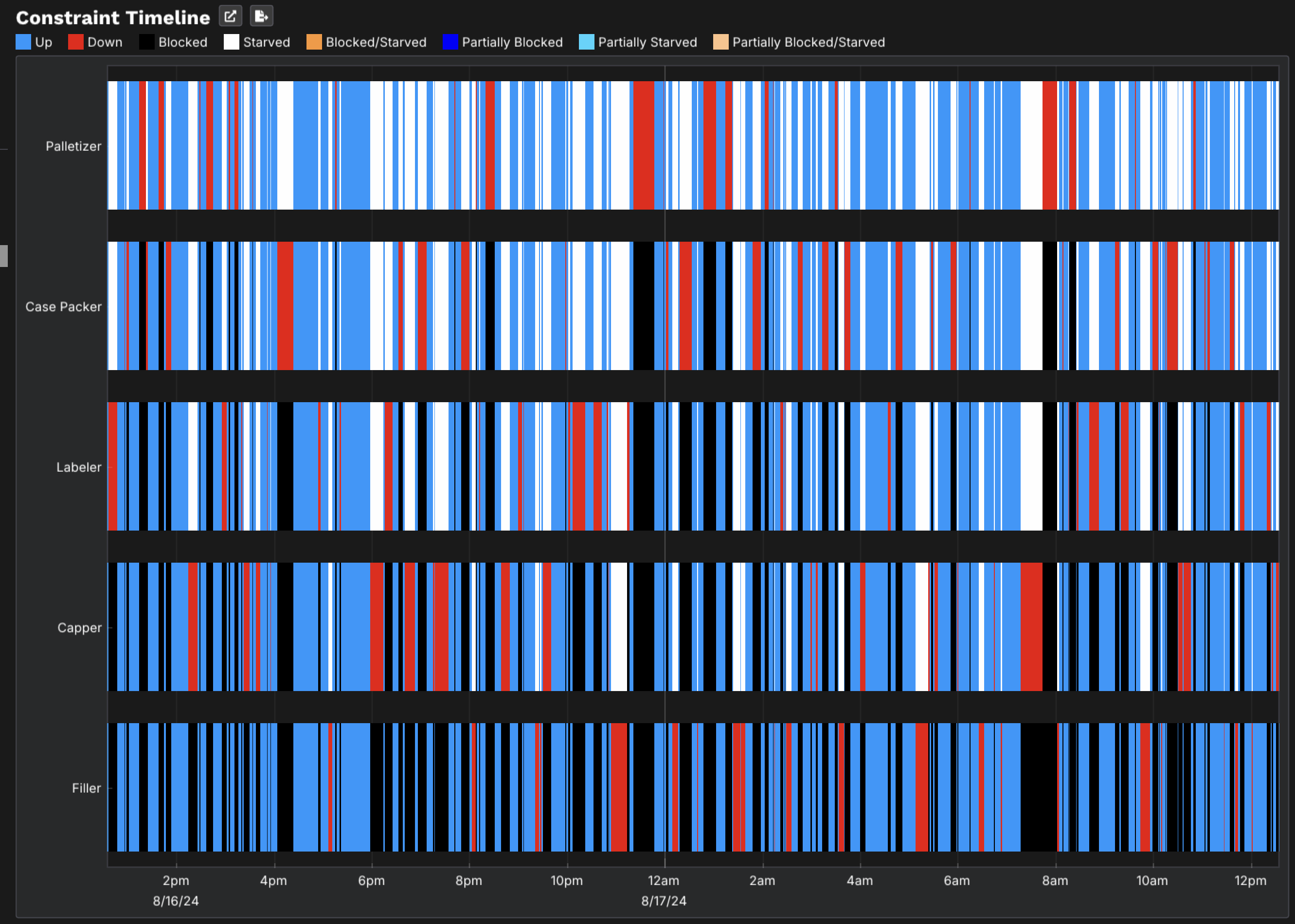
Step one is a distribution, not a name. The useful question is not “which machine is the constraint?” but “what share of the time is each machine the constraint, and under what conditions?” That is a question about how the line behaves through time — and it is the question a simulation answers directly.
Two plants where step one went wrong
The constraint that moved with the package
A quality initiative added a stage to an existing Make-Store-Pack coffee operation. The new stage was not the problem; scheduling was. As packaging sizes changed, the bottleneck moved, because a different format draws from the store at a different rate and shifts which stage is binding. The plant’s Advanced Planning System was optimising against a constraint that would not hold still.
A discrete rate model that reproduced the moving bottleneck, rather than assuming it away, let the team test and verify a new scheduling algorithm across a range of demand scenarios before deploying it. In TOC terms the model made step one honest — the constraint was identified per format, not once — and let step three be tested before it was trusted. The account is qualitative, from our project record: The Shifty Bottleneck.
The constraint everyone could see
At Bell-Carter Foods, an olive processor, the pitting machines took about two hours to change over between olive sizes — visible, expensive and apparently decisive. A capacity model of the whole plant found the binding constraints downstream instead, in packaging after the cans were filled and retorted. A Theory-of-Constraints daily schedule built on that finding recovered 15% more throughput with no new equipment. That work predates ReliaSim as a product; it was done by the same team with the same rate-based method, and it is written up in the Bell-Carter case study.
Step 1 by simulation: identify
Simulation replaces the walk-around with a measurement. Build the line with each machine’s rate and its real interrupts — time to failure and time to repair for each failure mode — plus the buffers and conveyors between machines. Run it over a horizon long enough to include the rare events as well as the common ones. Then read three things:
- Starved and blocked time per machine. The constraint is the machine that is neither — still running while everything around it waits. See Starved vs Blocked.
- Buffer levels. A buffer that runs chronically full points to a constraint downstream; chronically empty, upstream. See The Hidden Bottleneck.
- When each machine holds the role. The constraint timeline shows whether you have one dominant constraint or several machines trading it.
If one machine holds the role most of the time, classic TOC applies almost as written. If several share it, the steps apply to the set, and the “drum” has to be chosen deliberately.
Step 2: exploit — rank losses by what comes back
Exploiting the constraint means not wasting its time. On a production line most wasted constraint time is its own interrupts, plus the starvation and blocking its neighbours impose on it. The tempting shortcut is to attack the biggest downtime bar on the report. The measurement that holds up is different: remove one failure mode in the model, re-run the whole line, and read how much output comes back.
Those two numbers routinely disagree. In our bottling line case study, two failure modes had nearly identical direct losses. Removing the Filler micro-stops recovered 1.21× their recorded loss, because they had been cascading into the machines downstream; removing the Labeler misalignment recovered 0.73×, because part of that loss was already being absorbed. Which loss to fix first covers the method in full.
Step 3: subordinate — drum, buffer, rope
Drum–Buffer–Rope is TOC’s scheduling form of subordination. The drum is the constraint’s pace, which sets the rate for the whole line. The buffer protects the drum: stock placed ahead of the constraint so upstream stoppages do not starve it — in TOC it is sized and managed in time rather than in units. The rope ties material release to the drum, so the rest of the system does not overproduce into inventory the constraint cannot use.
On a continuous or high-speed line the buffer is physical: an accumulation table, a surge tank, an accumulating conveyor. Two consequences follow, and both are where simulation earns its keep.
- Protect both sides. A constraint loses time by being starved from upstream or blocked from downstream. Stock ahead of it covers the first; free space after it covers the second.
- Size on the stoppage distribution, not the average. A buffer covers a stoppage only while it has stock to give.
Illustrative example — not a result
| Quantity | Value | Meaning |
|---|---|---|
| Constraint draw rate | 60 / min | what drains the buffer |
| Typical upstream stoppage | 4 min | how long it must be covered |
| Buffer to cover it | 240 units | 60 × 4 |
| Double the buffer | 480 units | covers an 8-minute stop — worth little if few stops run that long |
Plot efficiency against buffer capacity and the curve always bends — steep, then flat — but where the knee falls is specific to the line. That is why buffer size should be swept rather than guessed. The Buffer-Options sweep in How big should a buffer be? — every capacity from 0 to 100 crossed with every interrupt, ten replications, 90 days — is 7,770 runs and finished in 31.8 seconds on a laptop. On that line the answer favours fixing the machine over adding storage, because the dominant loss is a long stoppage on the constraint itself and no buffer fills that. On a line with short, frequent stops either side of a well-protected constraint, the same experiment favours the buffer.
Step 4: elevate — and see where the constraint goes next
Elevation is where static TOC analysis is most likely to over-promise. Add capacity at the constraint and output rises only until the next-most-limiting resource starts to bind. After that, extra capacity at the old constraint produces nothing except more starved and blocked time elsewhere. The gain from elevating is the distance to the next constraint, not the size of the upgrade.
A model shows that distance before you pay for it. Raise the constraint’s rate or remove its dominant interrupt, re-run, and take the step-one readings again: which machine is now the constraint, how often, and how much output came back. If the next machine takes over almost immediately, the proposal is a two-machine project or a smaller one.
Watch for a machine that ends up mostly blocked. After an upgrade, a machine that spends most of its time blocked is making more than the next step can take. That is the model telling you the upgrade has already been used up.
Step 5: repeat — keep the model current
Goldratt’s warning about inertia is the step most often skipped. Product mix changes, a machine is rebuilt, a buffer is removed to free floor space — and the constraint moves without anyone announcing it. A line model kept current turns step five into a re-run rather than a new study.
That only works if the model is validated against the line’s own history, per failure mode rather than only in aggregate. The published reference point is Fischel and Lange’s WSC 2020 study, validated to within 1% of measured OEE over a one-year run — see Within 1% of measured OEE.
Why dice games and spreadsheets stop short
TOC is usually taught with a dice game or a capacity spreadsheet, and both teach the principle well: variability in a chain of dependent steps loses output, and the constraint governs. Neither can tell you about your line. A capacity spreadsheet takes each machine’s average rate and finds the minimum, which assumes the constraint is fixed and the variability averages out. A dice game has the right mechanism but none of your machines, failure modes or buffers.
Simulation keeps the mechanism and adds the specifics — each machine’s rate, each failure mode’s distribution, each buffer’s capacity — played forward through time. ReliaSim uses discrete rate simulation, which models flow as rates rather than individual items; Andy Siprelle originated the approach in 1990, and it is why sweeps like the one above finish in seconds.
Frequently asked questions
What is theory of constraints simulation?
Using a simulation model of a production system to carry out TOC’s five focusing steps by measurement rather than assumption: identifying which resource limits throughput and how often that changes, testing ways to exploit and protect it, and seeing where the constraint moves after it is elevated.
Can the bottleneck on a production line change?
Yes. On lines with breakdowns, buffers and a changing product mix, the active constraint shifts with which machine is down, which format is running and what the schedule takes out of the flow. A simulation run shows what share of the time each machine is the constraint.
What is drum-buffer-rope on a production line?
The drum is the constraint’s pace, which sets the rate for the line. The buffer is stock, measured in TOC as time, placed to protect the constraint from upstream stoppages. The rope ties material release to the constraint so the rest of the line does not overproduce.
How big should the buffer in front of the constraint be?
Big enough to cover the upstream stoppages that actually occur, sized on the distribution of stop durations rather than the average. Efficiency rises steeply with buffer capacity and then flattens; sweeping capacity in a model locates where it flattens on your line.
Does elevating the constraint always increase throughput?
Only until the next-most-limiting resource becomes the constraint. Past that point the extra capacity shows up as starved and blocked time elsewhere. Simulating the upgrade first shows how much output it buys before that happens.
Watch the constraint move
The ReliaSim Sandbox runs a bottling line in your browser. Stop a machine, change a buffer, and see which station limits the line. No signup.
Open the sandbox → The Shifty BottleneckWant to see it on a real line first? Read the case study — or schedule a call.