What Is Discrete Rate Simulation?
Model Flow as Rates, Not as Individual Events
Discrete rate simulation models a line as rates of flow between machines and buffers, instead of tracking every item. The simulator only does work when a rate changes. That makes it a natural fit for high-speed lines and bulk flow, where stops, buffers and blocking decide the answer. It’s the method ReliaSim® is built on.
The idea in one tank
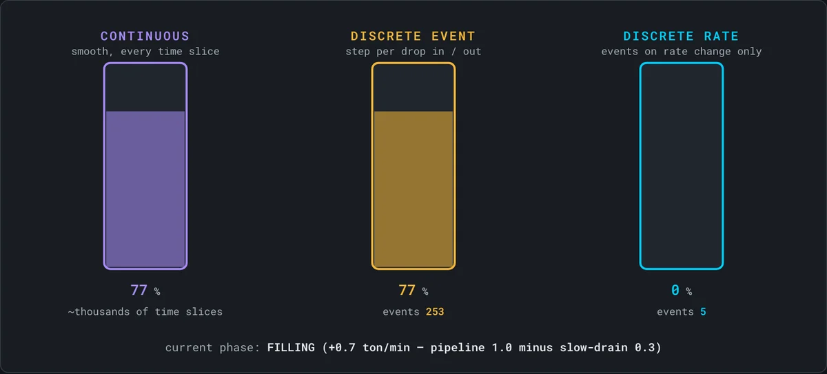
Fill a tank from a pipeline and drain it at a slower rate. A continuous simulation recalculates the level at every time slice, whether anything changed or not. A discrete event simulation steps once for every unit in or out. A discrete rate simulation fires an event only when a rate changes, such as the tank starting to fill, filling up or emptying.
Between those events the rates hold, so the level moves in a straight line and the simulator can compute exactly when the next change will happen. It does no work in between.
Scale that up to a real line and the gap grows with line speed. In the Hamburger Duo demo, a five-stage burger line runs as discrete event and discrete rate side by side, with 2,993 events against 6 for the same 300 burgers.
Three building blocks: constraints, buffers and interrupts
Every discrete rate model is built from three primitives. Any process you can describe as rates, accumulation and disturbances reduces to them.
Constraints
A constraint is any point that limits the rate of flow, such as a filler, a labeler, a reactor or a processing stage. Each has a maximum rate that can change over time. It runs at that rate until something changes it. An interrupt can slow it or stop it, a full buffer downstream can block it and an empty buffer upstream can starve it.
Examples: a filler at 1,200 cans a minute, a labeler at 850 bottles a minute, a reactor at 12 m³ an hour, a loading bay at 22 pallets an hour.
Buffers
A buffer is an accumulator between constraints. It fills when upstream runs faster than downstream and drains when downstream runs faster. Buffers are why a line doesn’t seize the moment one station hiccups. A well-placed buffer can absorb several minutes of downstream downtime, and a poorly sized one passes a stop straight through.
Examples: an accumulation table between filling and labeling, WIP between machining and assembly, a holding tank between a reactor and a distillation column.
Interrupts
An interrupt is an event that changes a constraint’s rate, such as a failure, a jam, a changeover, a quality hold or a scheduled stop. Each interrupt carries its own time-to-failure (TTF) and time-to-repair (TTR) distributions. A three-second label misread is one distribution and a four-hour belt replacement is another. Keeping them separate, instead of rolling them into one availability number, is how the model captures the knock-on effects that decide real-line throughput.
The three compose. A plant is a network of constraints connected through buffers and changed by interrupts, and the same three primitives describe a soap plant, a fuel pipeline or a distillation column.
Where event-by-event simulation struggles
Discrete event simulation makes each unit its own event. That’s the right choice when unit identity matters, and it gets expensive as line speed rises. A station running 1,200 units a minute fires 1,200 events a minute. The usual fix is to lump short stops into one downtime factor, which removes the blocking and starving that often decide what a fast line actually produces. Discrete rate vs discrete event simulation covers the comparison in full.
Where discrete rate simulation fits
It fits any system where material flows at a rate and interruptions disrupt that flow.
- Bottling and packaging. Filling, capping and labeling lines where a three-second stop spreads to the stations downstream.
- Food and dairy. Continuous flow with CIP cycles and quality windows, where buffer sizing affects product integrity as well as throughput.
- Pharma and life sciences. Tightly coupled, regulated processes where each interruption has to be modeled precisely.
- Chemical and continuous process. Reactors and columns where fouling lowers the rate gradually, which the model treats as an interrupt.
- Utilities and pipelines. Treatment stages with backwash cycles, generating plants with partial derating, and pipelines where line pack acts as the buffer.
- Beyond manufacturing. Fleets, logistics and hospital patient flow, where availability and rates change through the day.
Validated against a real plant
Fischel and Lange’s 2020 Winter Simulation Conference paper modeled a multi-line food plant in ExtendSim®. That model was rebuilt in ReliaSim and independently validated by Tom Lange, and the ReliaSim model came within 1% of both the plant’s measured OEE and the original model. The published OEE validation case study has the details.
How the method started
Andrew Siprelle created the technique in 1990, originally under the name bulk flow simulation. It entered the peer-reviewed record at the 1995 Winter Simulation Conference. The name discrete rate simulation came into use in the late 2000s, as the method was built into commercial simulation software.
Selected publications
| Year | Venue | Paper |
|---|---|---|
| 2020 | Winter Simulation Conference | High Accuracy Discrete Rate and Reliability Modeling to Drive Improvement of Plant OEE and Throughput (Fischel and Lange) |
| 2020 | ResearchGate | Mesoscopic Discrete-Rate-Based Simulation Models for Production and Logistics Planning |
| 2016 | Springer | Comparison of Discrete Rate Modeling and Discrete Event Simulation |
| 2014 | ResearchGate | A Global Approach for Discrete Rate Simulation |
| 2009 | Winter Simulation Conference | ExtendSim Advanced Technology: Discrete Rate Simulation (Krahl) |
| 1995 | Winter Simulation Conference | Modeling a Bulk Manufacturing System Using Extend (Siprelle and Parsons) |
More of the published record is on chiaha.com/research.
ExtendSim® is a registered trademark of Andritz Inc., referenced for identification only.
Guides on simulation methods
- Discrete rate vs discrete event simulation, including which tools use which method.
- Simulation methodologies, from discrete event to agent-based and system dynamics.
- Monte Carlo vs discrete rate simulation, and when a spreadsheet is enough.
- Digital twin vs simulation, and what a validated model is.
Frequently asked questions
What is discrete rate simulation?
Discrete rate simulation (DRS) models flow as a rate that changes only at discrete events, instead of tracking each unit as its own event. A model is built from constraints, buffers and interrupts. Between events the rates hold, so the simulator needs no recalculation until something changes.
How is discrete rate simulation different from discrete event simulation?
Discrete event simulation makes each unit an event the simulator schedules and processes, so its work grows with throughput. Discrete rate simulation makes each rate change an event (a failure, a repair, a changeover, a buffer filling or emptying), so its work grows with the number of rate changes instead of the number of units.
How is discrete rate simulation different from continuous simulation?
Continuous simulation integrates the state forward in small time steps whether anything changed or not. Discrete rate simulation is event-driven. It recalculates only when a rate changes or a buffer reaches full or empty, and because rates hold between events no numerical integration is needed.
What are the three primitives of discrete rate simulation?
Constraints limit the rate of flow. Buffers sit between constraints and absorb rate differences by filling and draining. Interrupts are events that change a constraint’s rate, each with its own time-to-failure and time-to-repair distributions.
What is bulk flow simulation?
Bulk flow simulation was the original name for discrete rate simulation. The 1995 Winter Simulation Conference paper that introduced it is titled Modeling a Bulk Manufacturing System Using Extend. The name discrete rate simulation came into use in the late 2000s.
Why is discrete rate simulation faster on high-speed lines?
In discrete event simulation a line running 1,200 units a minute produces 1,200 events a minute at each station. In discrete rate simulation the same line runs at a constant rate between interrupts, and the simulator does no work until a buffer fills, a failure fires or a changeover starts.
What software supports discrete rate simulation?
ReliaSim is ChiAha’s discrete rate simulator for production lines. ExtendSim offers discrete rate modeling in some editions. ChiAha’s free, browser-based Decoupling Buffer Simulator uses discrete rate simulation to explore buffer design.
Watch one tank run three ways
The Discrete Rate tier of the Sandbox runs the Fast-Slow Drain, the Hamburger Duo and five more models in your browser, with no signup.
Open the Fast-Slow Drain →Or compare the methods in discrete rate vs discrete event simulation.