From line event data to defensible throughput decisions — in minutes, not months.
ships with the modeling team built in. Your people get to the answer without hiring a simulation department — and every model is validated within 1% of your actual OEE.
Independently validated within 1% OEE — Tom Lange, 36 years Procter & Gamble
How do you increase production?
Every system has multiple ways to improve.
Add Buffer?
Improve Reliability?
Automate the Process?
How do you decide?
Gut feel?
Spreadsheets?
Past experience?
Consultants?
From raw data to prediction.
Distilling 35 years of the end-to-end process into three purposely parsimonious steps.
Build
Step 1
Sketch the line and parameterize each machine's behavior.
Simulate / Validate
Step 2
Run the baseline and match history within 1% before you predict tomorrow.
Decide
Step 3
Run what-ifs. Gain ≠ Loss. Act with numbers behind you.
Step 1 · Build → Sketch
Sketch what is.
Add equipment and operational details: units, rates, conversions, and buffers or decoupling points.
"It runs on my desktop. No integration, no IT project, no waiting." — Engineering Leader, Essity
Desktop-native by design — your production data never leaves your network. Air-gap compatible for OT, defense, and validated environments.
Every interrupt has two parts. The dice represent both.
Time to Failure
How long does the machine run before something goes wrong? Roll to find out.
Time to Repair
How long until the machine is back? Roll again. That's the whole interrupt.
TTF + TTR = one interrupt. Repeat until 7 days elapse. Five machines. When any one fails, the whole line stops.
Your handout
Roll d20 → look up minutes
d20
TTF
TTR
1
92
15
2
3
1
3
29
5
4
22
4
...
...
...
20
8
1
Same distribution, every team — just shuffled.
Mean TTF = 27.8 min · Mean TTR = 4.7 min
Same machines. Same distributions. What OEE will your team get?
Step 1 · Build → Parameterize
Compose your equipment behavior.
finds the shapes that fit each failure in your historian data.
Historical Line Event Data — blocking and starving emerge from the interaction
For systems without data, the Interrupt Designer guides your distribution selection based on your reliability process.
Infant Mortality
Decreasing failure rate
Wear-out
Age-related failures
Scheduled
Fixed-duration maintenance
Step 1 · Build → Fit with ReliaStats
Raw historian data → validated sim inputs.
ReliaStats fits the Time-To-Failure and Time-To-Repair distributions for every interrupt in your line — so the simulation runs on statistical reality, not guesses.
No historian data?
Start with the Interrupt Designer.
Pick the distribution shape that matches each failure mode from engineering knowledge — infant mortality, wear-out, random, or scheduled — and parameterize TTF + TTR directly.
Free, forever. No account. No upload. When historian data arrives later, ReliaStats fits it and swaps the distributions in place.
Eight distribution shapes
Weibull
LogNormal
Normal
Exponential
Uniform
Triangular
Johnson SU
Fixed
Five tools · one workspace
Interrupt Designer
Interrupt Validation
Interrupt Viewer
Interrupt Comparison
Interrupt FittingSubscription
Step 2 · Simulate / Validate → Match history
Validate against history. Within 1%.
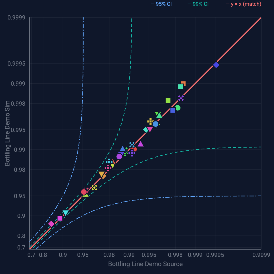
Model vs. historian
Each point is an interrupt. On the diagonal = model matches reality.
"The only way to predict this accurately is through simulation."
— Tom Lange, 36 years Procter & Gamble
Step 3 · Predict
Predict what ifs?
An ensemble of actors performing a thousand times.
Any durationRandom seed analysisSingle runMultiple runs
Step 3 · Decide → Experiment
What if?Gain≠Loss.
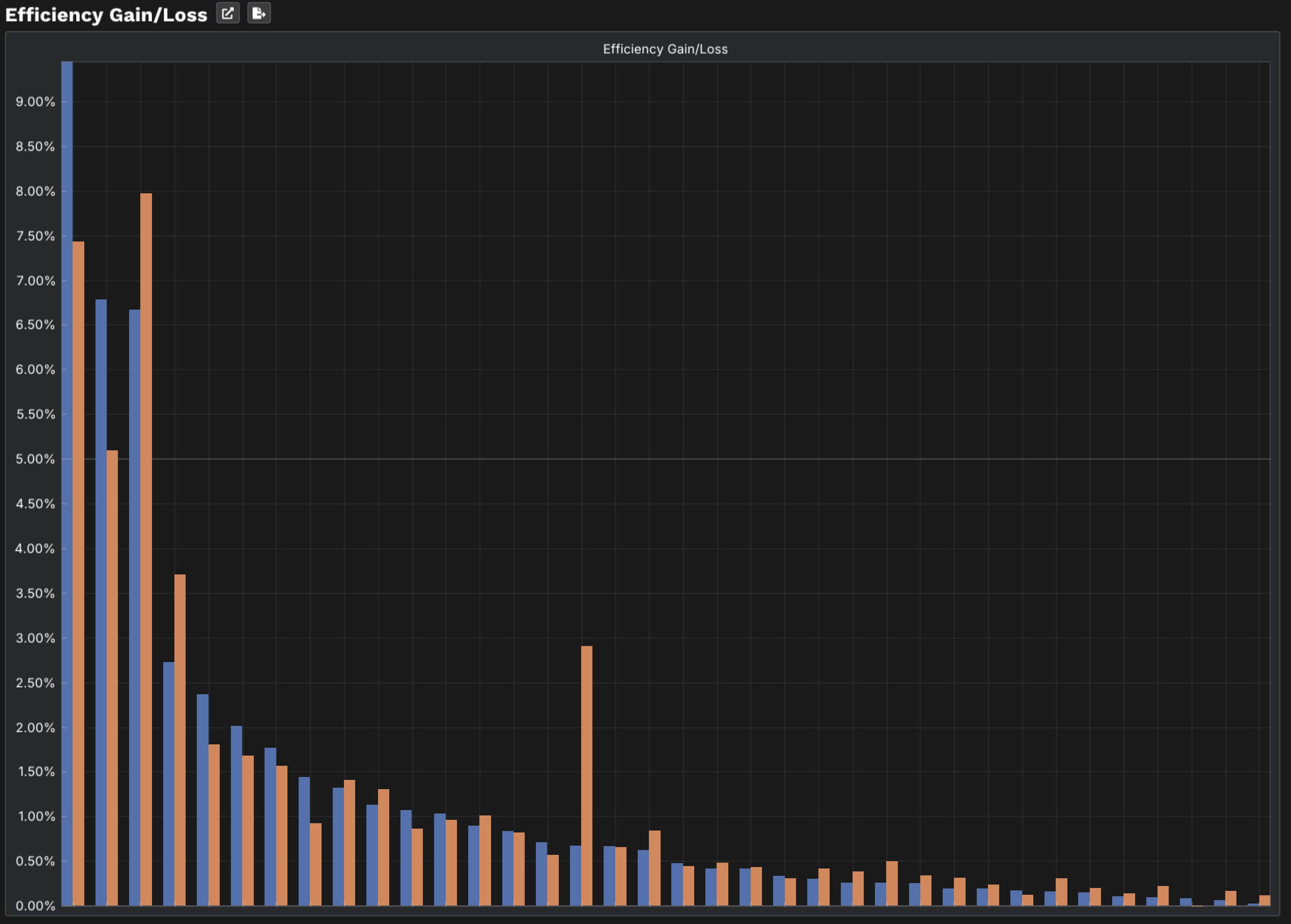
Eliminate each failure mode. Measure the whole system. The recovery is almost never equal to the loss.
Loss → Gain detail
Labeler Misalignment
Loss 6.78% → Gain 5.10%
0.75×
recover less than you lost
Filler Micro Stop
Loss 6.67% → Gain 7.97%
1.2×
56% more recovery
Same loss. Completely different recovery.
Step 3 · Decide → Act
Make confident decisions.
With the right tools in your toolbox, you can study 100 years of production in minutes.
🔧
Which failure first?
Rank by system gain, not downtime.
⚡
Faster or slower?
Faster = more product, more failures.
📦
How much buffer?
Protect the bottleneck — but how much?
🔁
Second machine?
Redundancy vs. reliability improvement.
🔄
Manual or auto resupply?
True cost is often 3× what downtime says.
🎯
The question your Loss Tree can't answer.
Every line has its own version.
AI-Powered via MCP
Ask your validated model anything.
Plain language questions. Simulation-backed answers. Powered by your specific validated production graph — not a generic AI.
🔍
Inspect topology & constraints
Node types, buffers, interrupt configs — in plain language.
MCP tools — works with Claude, any MCP-compatible AI, and Claude Code.
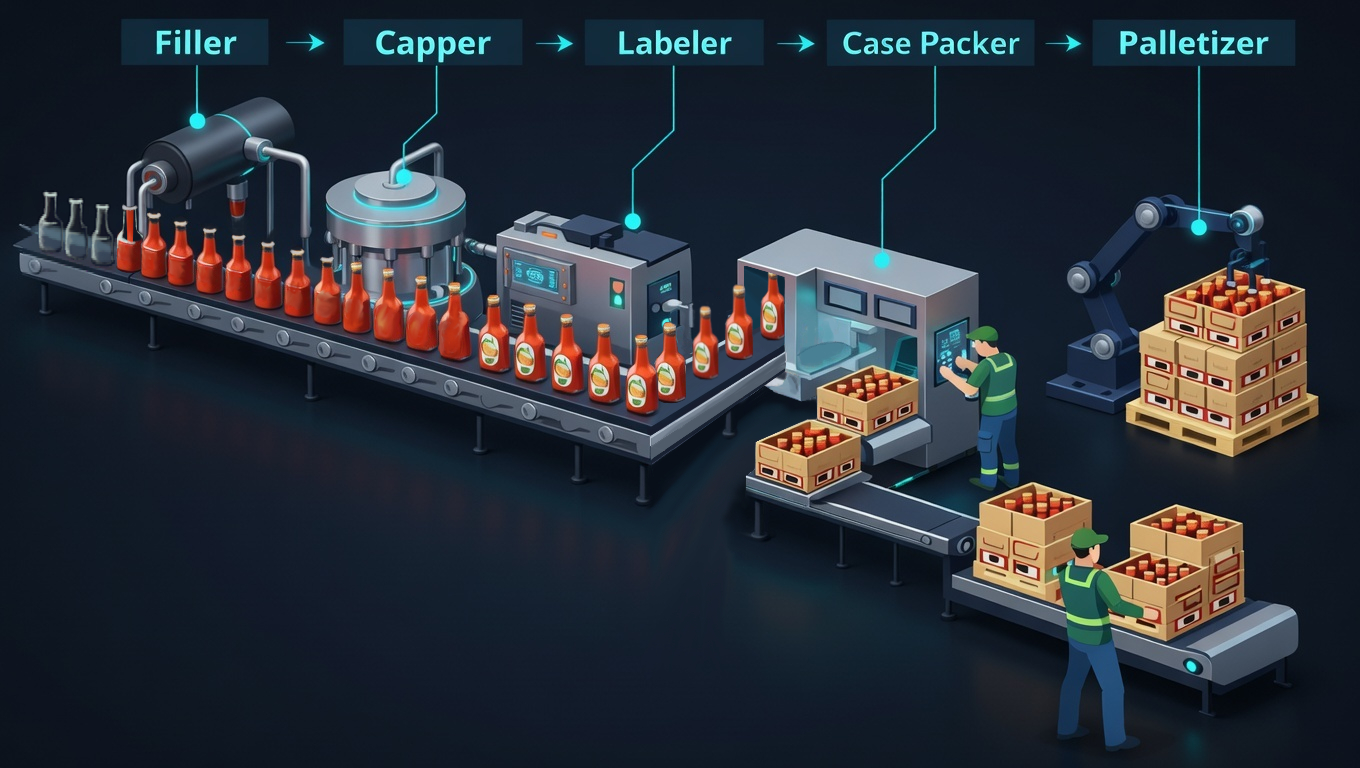
ReliaSim AI — Bottling LineValidated ✓
You
Using the Bottling Line model from Feb 1 – Mar 30, 2026 — what should I fix to improve OEE by 5%?
RS
The Capper is your critical path — 15,481 downtime events over 90 days with only 75.44% availability. Every outage starves three downstream machines. Start there.
You
Could a buffer before the Capper help?
RS
Yes — estimated +2–3% OEE at low capital cost. The buffer buys resilience; fixing the interrupts buys efficiency. Run both scenarios and compare.
You
Show me the top 5 interrupts by system gain.
RS
Top 5 by system-level gain when eliminated:
Capper Jam
7.97%
Filler Micro
5.10%
Labeler Align
3.21%
Packer Belt
2.14%
Palletizer
1.28%
Fixing the top two alone recovers +13.07% system gain.
Ask about throughput, buffers, interrupts…
+
See the impact of change before you make it.
~1%
OEE accuracy
15 min
Model construction
1,200×
Faster
300+
Organizations
"In my years at Pritsker, we came close to this, but we never made it work like this."
— Darrell Starks, Simulation Consultant, Integral Solutions
Trusted by production teams in 300+ organizations since 1995
Process Plus
Kellogg’s
Symbotic
JTEKT
Essity
Teleflex
Estée Lauder
Process Partners
+ 300 more organizations
Food & BeveragePharma & Life SciencesAerospace & DefenseEnergy & ChemicalPackaging & CPGPaper & PulpSemiconductorAcademic Research
Scan for the tour, podcast, and a 15-minute demo with your line.
chiaha.com
From bottling lines to warehouses.
Bigger scale — PlantSim modeling an end-to-end warehouse flow.
SiemensPlant Simulation · Authorized Reseller
Intelligent recommendations for your process.
Expert-level thermal process guidance delivered to operators in real-time — from raw PLC signals to a defensible process decision.
Enhance Operator PerformanceReduce Oven Fire RiskLower Energy Costs
Process Partners + ChiAha · Validated across 28,000+ data points
The problem is variability.
Every shift, every operator, every decision — different. The result: inconsistent product, wasted energy, and elevated fire risk.
Operators control complex thermal processes with dozens of variables
🔥
Fire Risk
Running hotter than necessary, provoking spark events
⚡
Energy Waste
Operators default to temperature as the only control point
📉
Quality Swings
Product density varies wildly between shifts
Real intelligence from basic science.
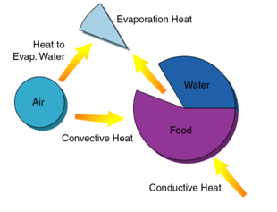
Not black-box AI. Dynamic mass-energy balance calculations — psychrometric modeling of air, water, food, and heat transfer.
Convective, conductive, and evaporative heat transfer — calculated in real-time
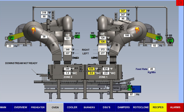
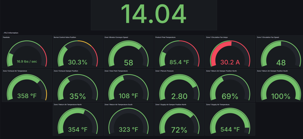
Live process monitoring — every variable, every second
Puffed Rice Oven Control
Impact on product density.
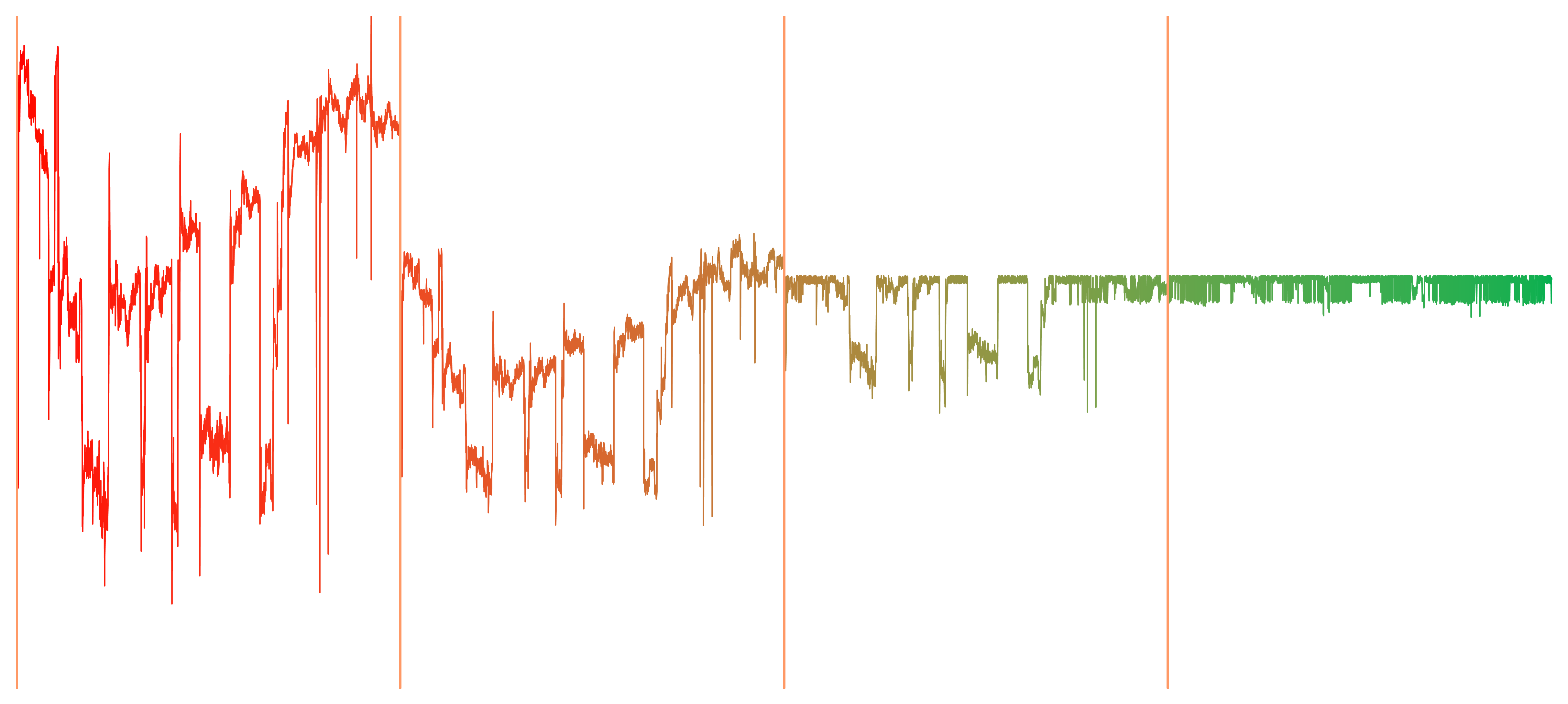
Each incremental iteration tightens
Operator Settings
AC Iteration 1
AC Iteration 2
AC Iteration 3
Product density variation ↓ 93% by iteration 3
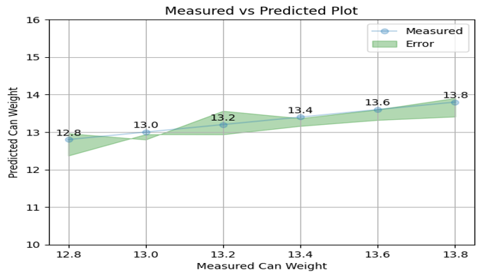
Validated across 28,000+ data points.
3% maximum prediction error — the model matches reality
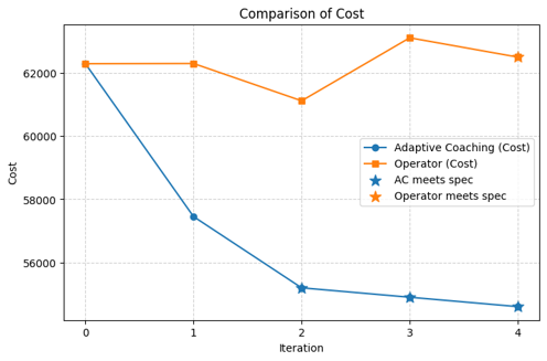
Energy cost drops with each iteration — operator cost stays flat
Puffed Rice Improvements.
0
Safety Incidents
13%
Energy Reduction
93%
Reduction in Std Dev
3%
Recorded Prediction Error
"The system monitors oven conditions, product density, and moisture levels to make live psychrometric calculations and then offers suggestions to operators to maintain target critical control points while utilizing the least energy."
— Plant Operations Manager
Where the value shows up.
Three categories of benefit — each tied to a specific Adaptive Coaching contribution.
Product Consistency
Fewer complaints — burnt or uneven.Oven balance visualized through the HMI.
Consistent between shifts.Recommended settings meet density targets 24/7.
Fewer underfill complaints.Density targets hit every run.
Safety
Reduced fire risk.Mass balance favors higher moisture, lower temperature.
Systematic load changes.Closed feedback loop on every adjustment.
24/7 safety visibility.Alert historian surfaces event history and durations.
Productivity & Cost
Higher OEE.Correct density reduces packaging stops.
Less overweight giveaway.No need to overfill to hit spec.
Lower natural gas use.Moisture-led operation cuts firing.
Faster expert collaboration.Curated settings shared with Process Partners.
How we start.
A three-step engagement — from onsite evaluation to live coaching.
1
Onsite Evaluation & Proposal
Understand your process and challenges — equipment readiness, NAFP inspection, optional workshop.
2
Install Adaptive Edge
Connect to the PLC to capture real-time operating behavior.
3
Design & Implement Adaptive Coaching
Build the psychrometric model for your process and deploy operator coaching.
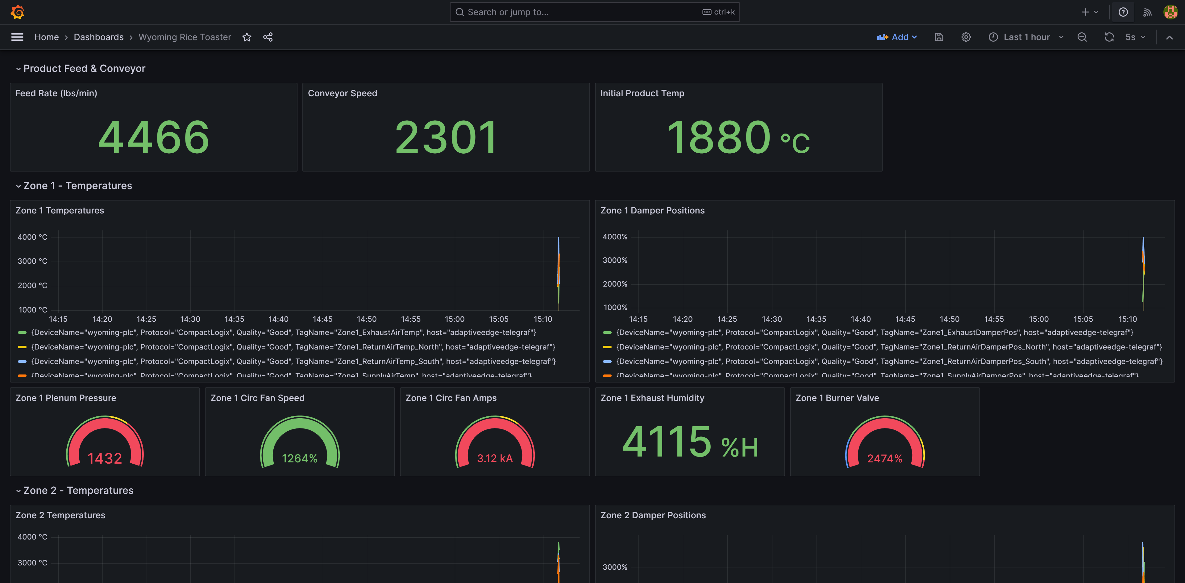
Air-gap capable PLC data acquisition on an industrial box PC. Time-series storage, live dashboards, and model-driven recommendations — all on your floor, behind your firewall.
<100ms
Read latency
1s
Poll interval
Request a PilotSee the Stack
adaptive-edge.com
Supply chain network design · no consultant required
Find your optimal DC locations in minutes, not months.
See how GIS-enhanced facility siting works on sample data in minutes. No six-figure consulting engagement. No bloated enterprise software license.
• No data stored• No credit card required• Built by supply chain veterans
80%
of enterprise tool value, at a fraction of the cost
 +
+


 Bulk Storage
 Filler A
 Capper A